Date Manipulation in SAS

I need to produce a report that contains historical data of some sort based it's Tuesday snapshots in the year 2009 and 2010.  Then I found this Intnx function to help.  For example:

To get a list of Tuesdays starting Jan 6, 2010 into a dataset called tuesdays:

%let start_date='06jan2009'd;
data tuesdays ;
do i = 0 to 103;
    Tuesday=put(Intnx( 'Day' , &start_date ., i*7 ),date9.);
    output;
end;
drop i;
run ;
proc print data=tuesdays; run;

To load all Tuesday's SAS data files:

%let start_date='06jan2009'd;
%macro load_tuesday_sas_dataset;
    %global tuedate;
    %do i=0 %to 103;
        data _null_;
            call symput("tuedate",left(put(Intnx('Day',&start_date., &i. * 7),date9.)));
        run;
        %put &tuedate;
        data dataset_&tuedate.;
            set filelib.sasfile_&tuedate.;
        run;
    %end;
%mend load_tuesday_sas_dataset;
%load_tuesday_sas_dataset;

Enjoy learning SAS, a little bit at a time every day.

Reading Excel and Access files on SAS 64-bit

Finally got my machine rebuilt to Windows 7 64-bit, and had SAS 9.2.3 64-bit loaded.  Then I started to have problems running some SAS code to read Excel and Access files.  Error message is:

ERROR: Error trying to establish connection: Unable to create Data Source.: Class not
       registered
ERROR: Error in the LIBNAME statement.

The original SAS code for reading Excel and Access files are as follows:

libname xlsfile oledb init_string="Provider=Microsoft.ACE.OLEDB.12.0; Data source=c:\temp\ExcelFile.xlsx; extended Properties=Excel 12.0";

libname accfile oledb init_string="Provider=Microsoft.ACE.OLEDB.12.0; Data Source=c:\temp\AccessFile.accdb; Persist Security Info=True";

Working with SAS technical support, I found that our tech guy installed Office 32-bit on my machine.  SAS 64-bit could not use the 32-bit Office drivers.  But what I understand from technical support was even if I had Office 64-bit installed, I still would encounter some issues because 64-bit is officially supported in SAS version 9.3.  They mentioned something called PC Server that could help me.  I read up about it online, and eventually found a solution.

First, I have to install SAS PC Server component on my machine.  Then I need to change the SAS code to the followings accordingly:

libname xlsfile pcfiles type=Excel port=8621 server=localhost path = "c:\temp\ExcelFile.xlsx";

libname accfile pcfiles type=Access port=8621 server=localhost path = "c:\temp\AccessFile.accdb";

Thanks to this article DID YOU KNOW THAT YOU CAN NOW ACCESS PC FILES ON A WINDOWS MACHINE DIRECTLY FROM A UNIX MACHINE? which helped me solve the problem.

To Escape % Character in SAS PROC SQL

Suppose you want to run a query to find all records containing the pattern "REQUIRED" in a certain column, the SQL where clause will look something as follows:

where thetextfield like "%REQUIRED%"

But if you use it inside SAS, SAS will interpret the %REQUIRED as a macro and throw an error.  Here is how you can escape the % character:

%let pattern=%nrstr(%%)REQUIRED%str(%%);
proc sql;
create table new_dataset as
select * from dataset
where thetextfield like "&pattern.";
quit;

You can also put the code inside a macro, and have the pattern "REQUIRED", etc as a parameter to be passed into the macro.

%macro get_records_with_pattern(pattern);
    %let patternlike=%nrstr(%%)&pattern.%str(%%);
    proc sql;
    create table new_dataset as
    select * from dataset
    where thetextfield like "&patternlike.";
    quit;
%mend get_records_with_pattern;

Now you can call the macro with the parameter REQUIRED and many more.

%get_records_with_pattern(REQUIRED);
%get_records_with_pattern(ACCEPTED);
%get_records_with_pattern(PASSED);

Calculating Cumulative Percentage In PROC REPORT With ACROSS

I am finally able to get cumulative percentages calculated when /across is used in PROC REPORT.  Basically I have to programmatically calculate it in the code, and put the resulting value into the columns directly (such as _c4_ for column 4, _c7_ for column 7).  I contacted SAS technical support on this, and confirmed there was no way around this hard-coding of column number.  How sad!

Here is the SAS code, with column numbers hard-coded, but at least it works:

options missing=0;
proc report data = some_dataset nowd missing;
column credit_load snapshotdate,(ones ones=onespct cumpct) dummy;
define credit_load        / group 'Credit Load' ;
define snapshotdate     / across '' order=internal;
define ones                     / analysis sum 'Freq' style(column)={tagattr="format:##0"}    ;
define onespct               / analysis pctn 'Pct' style(column)={tagattr="format:##0.0%"};
define cumpct               / 'Cum Pct' style(column)={tagattr="format:##0.0%"};
define dummy              / noprint;

COMPUTE BEFORE ;
    cumtot1 = 0;
    cumtot2 = 0;
ENDCOMP;

COMPUTE dummy;
    cumtot1 + _c3_;
    cumtot2 + _c6_;

    _c4_ = cumtot1;
    _c7_ =  cumtot2;

    IF _BREAK_="_RBREAK_" THEN DO;
      _c4_=1;
      _c7_=1;
    END;
ENDCOMP;

rbreak after / summarize ;

run;

Mathematica Box and Whisker Plot

I am trying to find a visualization to describe the distribution of our assessement data.  With a box and whisker plot, I can show the five statistical summary (minimum, maximum, first quartile, median and third quartile) in one chart.  I can create a chart for each assessment dimension, and put them side by side together.

It is surprisingly easy to do it programmatically in Mathematica,  Starting with a list of ratings (raters, ratings of dimension 1, 2, 3 and 4), then one single line of code using BoxWhiskerPlot function.  That's it!

BoxWhiskerPlot[
 Select[ratings[[All, 2]], NumberQ],
 Select[ratings[[All, 3]], NumberQ],
 Select[ratings[[All, 4]], NumberQ],
 Select[ratings[[All, 5]], NumberQ],
 BoxLabels -> {Style[dimensionnames[[1]], 11,
    FontFamily -> "Tahoma"],
   Style[dimensionnames[[2]], 11, FontFamily -> "Tahoma"],
   Style[dimensionnames[[3]], 11, FontFamily -> "Tahoma"],
   Style[dimensionnames[[4]], 11, FontFamily -> "Tahoma"]},
 BoxFillingStyle -> {RGBColor[0.3, 0.6, 0.9, 1],
   RGBColor[0.5, 0.7, 0.3, 1], RGBColor[1, 0.5, 0, 1],
   RGBColor[0.71, 0.22, 0.26, 1]},
 PlotLabel ->
  Style[DisplayForm[
    GridBox[{{"Assessment 2010"}, {"Box covering 50% of data (N=" ~~
        ToString[Nsize] ~~ "Programs)"}, {" "}}]], "Title", 14],
 FrameLabel -> {None, Style["Ratings", 11, FontFamily -> "Tahoma"]},
 BoxOutliers -> Automatic,
 PlotRange -> {Automatic, {0, 6.5}},
 ImageSize -> {520, 300}]
 

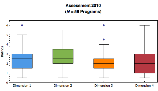
Mathematica also has an option to choose whether to show outliers.

I have created a lot more different kinds of visualizations, including an interactive sector chart.  Thanks to the Mathematica's Manipulate (or the MSPManipulate in webMathematica) function.  I will post them here when I have more time.

Mathematica, I am loving it!

Mathematica Bubble Chart

I was trying to show correlation between two dimensions visually in an assessment project.  I didn't feel the regular plot would do enough justice since the dots that overlap only count as 1.  So I experimented in using the bubble chart in Mathematica.

Here is the code:

ratingpairstally = Tally[ratingpairs];
bubbledata = {};
For[i = 1, i <= Length[ratingpairstally], i++,
  AppendTo[bubbledata,
    Join[ratingpairstally[[i, 1]], {ratingpairstally[[i, 2]]}]];
  ];

Show[
    Plot[{fitline}, {x, 0, 6},
  PlotLabel ->
   Style[DisplayForm[
     GridBox[{{"Assessment 2010"}, {dimensionnames[[1]] ~~ " vs " ~~
         dimensionnames[[4]] ~~ "(" ~~ ToString[Nsize] ~~
         "Programs)"}, {" "}}]], "Title", 14],
  AxesLabel -> {Style[dimensionnames[[4]], 11,
     FontFamily -> "Tahoma"],
    Style[dimensionnames[[1]], 11, FontFamily -> "Tahoma"]},
  PlotStyle -> Gray,
  PlotRange -> {{0, 6.5}, {0, 6.5}},
  AspectRatio -> Automatic,
  ImageSize -> {350, 350}]
 ,
 BubbleChart[bubbledata,
  ChartStyle -> RGBColor[0.3, 0.6, 0.9, 1]]
 ]

Basically, I have pairs of ratings stored in a list called ratingpairs.  I then used the Tally function to get the count of all distinct value of rating pairs.  Formatted the output properly into another list called bubbledata, ready to be plotted.  I use the Show function so I can put the bubble chart, and the line of best fit together.  Viola!
 

Radar Chart Gadget verified by Google - Yeah!

Google now requires all custom gadgets to be verified by them in order they can be viewed by collaborators. Refer to the Gadgets: Verifying Custom Gadget Google docs help page for more information.

I had developed a Radar Chart Google Spreadsheet Gadget a while ago. And our department have been using it to visualize the assessment data. So I better submit it to Google for verification as soon as possible.

It took about 3 business days... and YES! As of noon today, Google had verified my radar chart gadget. I hope it will be listed in their gadget gallery soon.